Maths
Various notes (crib sheet) from trying to understand various things... really just stuff you'd find in any old math text book. Oh and this is a useful MathJax reference on StackExchange. And Detxify can be used to draw the symbol you're looking for! For an interactive view of your mathjax try here. For graphing functions try Desmos.
Page Contents
References and Resources
The following are absolutely amazing, completely free, well taught resources that just put things in plain English and make concepts that much easier to understand! Definitely worth a look!
- The amazing Khan Achademy.
- The amazing CK12 Foundation.
For a more in-depth look at calculus the following book is AMAZING! Written really well. I wish I'd had this book when I was at school!
- The Calculus Lifesaver, Adrian Banner.
Also, not free, but still looks good and encourages learning by problem solving, is the excellent Brialliant.org.
Oooh and this guy's animations look pretty cool too.
Todo / To Read
https://math.stackexchange.com/questions/706282/how-are-the-taylor-series-derived
Laplace Transform Explained and Visualized Intuitively - https://www.youtube.com/watch?v=6MXMDrs6ZmA
Derivatives of exponentials | Chapter 5, Essence of calculus - https://www.youtube.com/watch?v=m2MIpDrF7Es
The Laplace Transform - A Graphical Approach - https://www.youtube.com/watch?v=ZGPtPkTft8g
Function Scaling
Partial fractions
The point of partial fractions is to do the reverse of:
In other words, given the following, Partial fractions let us go back to, We would start this by first factoring the above to get, We know that we want to get to something like, We can remove the denominators by multiplying through by to give, Matching terms between and , we get, Solving these simultaneous linear equations, we get, And so we can get back to Yucky example, sorry!
Summary Of Partial Fraction Rules
- Numerator must be lower degree than denominator. If not, then first divide out.
- Factorise denominator into its prime factors.
- A linear factor gives partial fraction
- A repeated factor gives
- Similarly gives
- A quadratic factor gives
- A repeated quadratic factor gives
For example, Has partial fractions of the form...
Difference Of Two Cubes
So for example...
Trigonometry
Wikipedia has a nice list of proofs for these :)
The "cut the knot" website lists some excellent proofs of the fundamental Pythagorean Theorem
Basics
Some trig functions are "complementary" in the sense that a in pair of such functions, one equals the other shifted by 90 degrees ( radians). So, "cos" is "complementary sine", for example, and "cot" is "complementary tan". The one that doesn't quite fit this pattern is the "csc" and "sec" complements :'(...
Radians
Here is a fantastic page about the why of radians. In summary radians define a circle such that the angle measured in radians is also the arc length around the unit circle for that arc.
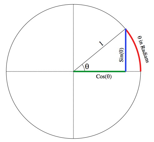
[Image taken from Ask A Mathamatition.]
Common Values For Sine and Cosine
Reference Angles and the ATSC Method
Sum and product formulas
Reduction Formulas
Pythagorean Identities
Sum or Difference of Two Angles
Double Angle Formulas
A Nice GIF Relating Sin And Cos

Found the above here.
Logarithms
Series
Basic Series
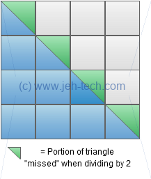 Consider summing the numbers in the series . For each number in the series, imagine stacking blocks to the left of the last stack.... you'd build up the triangle shown to the left. It's basically one half of a square. Trouble is if you divide the square by 2 you would chop off the top half of each block at the top of its stack. Therefore for each number in the series you have "lost" half a block.
Therefore the total number of blocks is... Where is half of the square and is the total of all the halves that we "cut" off (but didn't mean to) when we took the half.
Therefore, we can say... And...
Arithmetic Progression
Geometric Progression
If , then as , , Or, if (useful for the z-transform), then
Binomial Theorem
The binomial theorem is summarised as... Where the nth term is given by the following equation.
Exponential Series
The exponential series is defined as... This is why
The constant can be expanded as follows... And powers of as ...
Malclauren's Theorem
Attempts to express a function as a polynomial.
Note that the series must be shown to converge.
Need to figure out the coefficients. Notice the following.
Notice then...
And so on...
It thus looks like, and indeed is the case, that:
The above definition can then be used to derive the expansion of , which is why we were able to say: Remember, the series must be shown to converge! This is easily seen because the denominator is growing at a faster rate than the numerator.
Using this we can derive Euler's Formula.
Summing the above two expansions we get... Doing a similar expansion for we get the following and can then see how we get Euler's formula...
Imaginary & Complex Numbers
Intro
The definition of a imaginary number, , is , which is also often seen written as . It's called "imaginary" because the square root of -1 doesn't exist in real terms: there is no real number that when multiplied by itself is negative. Thus, the set of real numbers has been "extended". Sometimes is used instead of to denote an imaginary number.
A complex number is one that has a real and imaginary part, even if the real part is zero. Thus real numbers are a subset of complex numbers.
Rectangular Form
In rectangular form we write complex numbers like this: , where and are real numbers. If then it we can write and .
The representation of a complex number as is called rectangular form.
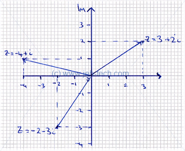
A complex number can be viewed graphically on an argand diagram, which is a little like a Cartesian diagram, except the horizontal axis is the real component and the vertical axis is the imaginary component of the complex number:
| Add | |
| Subtract | |
| Multiply | |
| Divide | Need complex conjugates for this. See below... |
Complex conjugates. The complex conjugate of is defined as (where and are just two different notations that mean the same thing). The can be visualised as shown below:
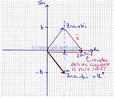
The next thing to talk about is the magnitude of a complex number. In the above diagrams we can see that the vector forms a right-angled triangle with the horizontal axis. The magnitude is the length of the vector and this is defined as follows:
Polar Form
Complex numbers can also be written in polar form by specifying magnitude (distance from the origin) and angle...
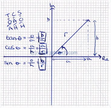
How do we go from rectangular form () to polar form ()? Recall and that therefore . We already know row to calculate .
Lets do a quick example. Let : Thus, in polar form the complex number is expressed as .
Exponential Form
From polar form we go to exponential form. This means that we can re-write as And using Euler's amazing formula , we can write... This is the exponential form. It is especially useful if you want to do division of complex numbers.
We can go back from exponential form to rectangular form using the same two formulas we saw above: and .
Taking the example from the previous section where we saw that we could represent as , we can now see this is easily converted to exponential form: .
And, if we wish to go back we can see that (approximately because the 0.983 value is rounded).
The exponential form is particularly useful in subjects like DSP for doing things like changing a signal's phase, which ends up just being a multiplication like this: The number is rotated anticlockwise by radians!
To explain a little more clearly, a discrete complex exponential is generally represented as: Where is the angular frequency is radians per sample period, is the amplitude and is the initial phase of the signal in radians. If we had to do a phase shift of the signal we'd either have to remember a whole load of trig identities or use the complex exponetial form, which makes life easier...
We can see this very simply by noting the following: The phase shift has become just multiplication.
Combinations & Permutations
Selecting samples from a set of samples at random. If the order of the elements matters then it is a permutation, otherwise it is a combination. If I have a set of objects and I select objects, on the first selections I can choose from objects. For the second selection I can choose from objects. This looks like the beginning of a factorial, but the factorial would look like this. We only want the first 2 terms. To get rid of the remaining terms we need to divide by , in other words, . Hence the formula above.
With combinations the order is not important. This time take ... for every choice I make there will be permutations with the same elements, which is one combination (as order is now not important). This is the case because the 3 elements can be ordered any how and count as the same object. and are, for example, no different. Out of all sets containing only these elements there must be permutations. Therefore need to get rid of this count from by divifing by in the general case...
For a fairly explicit example of combinations v.s. permutations and their application in statistics see this little example.
Square Roots
Reference: Mathwords.
Limits
Definition
When we talking about the limit of a function, we are asking what value the function will give as the input gets closer and closer to some value, but without reaching that value. The animation below tries to explain this:
What you should see in the animation is that we can always get closer to the point without ever reaching by adding smaller and smaller amounts. In other words, you can get as close to the limit (in the above case 9) by getting sufficiently close to some input (in the above case 3)
Intuitively, If is defined near, but not necessarily at, , then will approach as approaches . More rigorously, let be defined at all in an open interval containing , except possibly at itself. Then, If and only if for each , there exists such that if then .
I.e., no matter how close to we get, there is always a value of arbitrarily close to the limit value, , but which is not , that yields this value close to .
Ie. We can pick a window around the y-axis value and if we keep shrinking this window, we will always find an value, either side of that will yield a y-value in this error window. So, the error can be arbitrarily small and we will always find an either side of to satisfy it :) This is the two sided limit.
Limit Properties
Most of these are only true when the limits are finite...
| Uniquness: | If and then |
| Addition: | |
| Scalar multiplication: | |
| Multiplication: | |
| Division: | |
| Powers: |
Ways To "Solve" Limits
If the limit is not of the form , i.e., tends to some known number, first try pluggin that number into the equation. If you get a determinate answer thats great.
Generally though we get an indeterminate answer because we get a divide by zero...
If you can transform the function you're taking the limit of to something where there is no longer a divide by zero, note that original function and the transform are not exactly identical. Let's say the original function is and you have transformed it to .
If and at is indeterminate, our transform to is not. This means and are not the same function. But because limits are only concerned with values near and not at , this is okay as the functions are identical everywhere else.
When numerator non-zero but denominator zero, there is at least one vertical asymptote in your function. Either the limit will exist here or you will only have a left or right sided limit if on one side the y-axis tends in the opposite direction to the other side of the asymptote.
Factor Everything
If then factor to and cancel out the denominator. You can also use the difference of two cubes to help with more complex functions: .
Get Rid Of Square Roots
For problems where , where a is not you get rid of square roots by multiplying by the conjugate. If you have you multiply by . If you have you multiply by : Now when , hopefully you won't have an indeterminate fraction!
Rational Functions
When , the leading term dominates. If then the leading term is . Putting , we say that... This does not mean that ever equals , just that the ratio of the two tends to one as tends to infinity!
If you are taking the limit of a rational function like the one below... ... you can't just substitute infinity for because you get which doesn't make a lot of sense...
So do this... We know that because the leading term dominates... Which means that we will really be looking at the limit of... ... as tends to infinity!
A numerical example. Solve So we do... Everything tends to one except , which is equal to , so we know that this tends to zero!
In general, for our polynomials and :
- If degree of n == degree of d, then limit is finite and nonzero as
- If degree of n > degree of d, then limit is or as as
- If degree of n < degree of d, then limit is 0 as
N-th Roots...
When there are square roots, or indeed n-th roots in the equation the leading term idea still works. All that happens is that when you divide the n-th root by the leading term you bring it back under the square root.
Be careful when because when is negative! It equals . Use the following rule. If you write... You need a minus in front of when is even and is odd.
The Sandwich Principle / Squeeze Theorem
If for all x near a, and , then too.
Sal on Khan Achademy gives a good example of using the squeeze theorem to solve the following limit. The limit cannot be defined at , so the function is not continuous at that point, but it can still have a limit as tends to 0, as it does not have to equal 0... we only have to be able to get arbitrarily close.
L'Hopital's Rule
Can be summarised as follows... L'Hopital's rule can be used when the normal limit is indeterminate. For example... Substituting in gives , which is indeterminate. So, apply L'Hopital's rule by differentiating numerator and denominator separately... Substitute in for gives . Therefore...
Trig functions
For small values of , and are approximately the same. For really small values, I'm not even sure my computer has enough precision to be able to accurately show the difference. But, using a small python script we can get the idea:
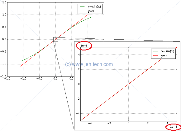
The above image was generated using the following script:
import matplotlib.pyplot as pl
import numpy as np

x = np.arange(-0.0001,0.0001, 0.000001)
y_lin = x
y_sin = np.sin(x)

pl.plot(x,y_sin, color="green")
pl.plot(x,y_lin, color="red")
pl.grid()
pl.legend(['y=sin(x)', 'y=x'])
pl.show()
In fact if your print(y_sin/y_lin) you just get an array of 1's because the computer does
not have the precision to do any better. I think even at small values of it is not the case
that , but it is very close. So in reality, even for tiny :
But, the following does hold:
The following also hold:
"Continuous" In Terms Of Limits
Continuous At A Point
A function is continuous at a point if it can "be drawn without taking the pen off the paper" [Ref]. This means, more formally, that a function is continuous at if .
As Adrian Banner says in his book "The Calculus Lifesaver", it is continuity that connects the "near" with the "at" in terms of limits. It is what allows us to find limits by direct substitution.
Continuity Over An Interval
If a function is continuous over the interval [a, b]:
- The function is continuous at over point in (a,b).
- The function is right-continuous at x = a: and exists.
- The function is left-continuous at x = b: and exists.
Intermediate Value Theorem
If is a function continuous at every point of the interval , then:
- will take on every value between and over the interval, and
- For any between the values and , there exists a such that
Min/Max Theorem
If is continuous on [a,b], then has at least one maximum and one minimum on [a,b].
Differentiation
Definition
Recall that a function is continuous at a point if it can "be drawn without taking the pen off the paper" [Ref]. This means, more formally, that a function is continuous at if . For a function to be differentiable at a point, it must be continuous at that point....
The derivative of a function with respect to it's variable is defined by the following limit, assuming that limit exists. If the limit does not exist the function does not have a derivative at that point.
This is why, for example the function does not have a defined derivative at , because the limit (of the differentiation) does not exist at that point. The function is continuous at that point because the left and right limits are the same, but the derivative function does not exist.
A function is continuous over an interval if:
- it is continuous at every point in ,
- it is right-continuous at , i.e.,
- it is left-continuous at , i.e.,
If a function is differentiable then it must also be continuous.
If is replaced with we would write Where just means a "small change in". This small change in leads to a small change in , which is given by . Therefore we can write: I.e, if can be written as .
Now at school, as we'll see in the integration by parts section, sometimes was treated as a fraction although my teacher always said that it wasn't a fraction. The above, which I didn't know at the time, explains why. And, finally, in the awesome book "The Calculus Lifesaver" by Adrian Banner [Ref] I know why :)
Unfortunately neither or means anything by itself ...
... the quantity is not actually a fraction at all - it's the limit of the fraction as .
Example
We can use the definition above to take the derivative of : We know that this limit exists because the function is continuous by virtue of it being a polynomial. We also know that is tending to zero, so those terms just dissapear, which leaves us with... Thus,
Basic Differential Coefficients
Chain Rule
Using this when you need to differentiate a function that is made up of the result of one function passed into the next and so on. I.e. if .
Quotient Rule
When you have a function that can be expressed as a fraction, use the quotient rule to allow you do differentiate and independently (easier!) and the combine the results using this rule. becomes and becomes :
Example
Solve the following: To do this we note that it is of the form where: So we can calculate: Plugging these into the quotient rule formula we get,
Product Rule
Use the product rule when trying to differentiate a quantity that is the multiplication of two function. I.e when trying to find the derivative of when . One of these functions becomes , the other . Use this so you can differentiate the simpler functions and independently and then combine the results.
For two functions...
Or for three functions...
Or, even, for any number of funtions...
... add up the group times and put a in front of a different variable in each term ...
The following is a really cool visual tutorial by Eugene Khutoryansky...
Example
A fairly simple example - find the derivative of . Okay, so we could just expand this out but it would be pretty tedious. The product rule help make it easier!
In this case if we let and , then we can write , which is in the exact pattern we need for the product rule where we will label as and as : We can find their derivatives as follows. Let . And ... Therefore... Let . And... Therefore... Now that we have the above we can use the product rule:
Integration
Basic Integrals
Integration Of Linear Factors
Use variable substitution, for example, if the integral is Then put , giving... But now we need to integrate with respect to , not !. In other words we need to go from the above integral to something like, We can use the chain rule as follows... By integrating both sides of the equation with respect to we get.... We now have an integral of some function with respect to . We can find from the definition of the original integral (just differentiate both sides!). We can find by firstly rearranging to... Then take the derivative with respect to to get Notice how, that because the "thing" (factor) that is raised to a power in the integral is a linear function, the terms will always dissapear, leaving only a constant, which can be differentiated w.r.t . If terms remained after differentiating the "thing" (factor), it would stop us doing our desired integration w.r.t ! Now we can see that... Substitute this into our integral and we have... This we know how to integrate the above using the list of standard integrals. Now we can substitute back in for to obtain the answer
One point to note is as follows. I always remember being taught to re-arrange the substitution that was made... To... ..And then subsitute for the term in the integral. However, this is not strictly correct as far as I understand because a differential coefficient is not a fraction... it is a limit: So, as we can see is not really a fraction... hence the above method and explanation, even if the "trick" I was taught works.
Integration By Parts
Phasors
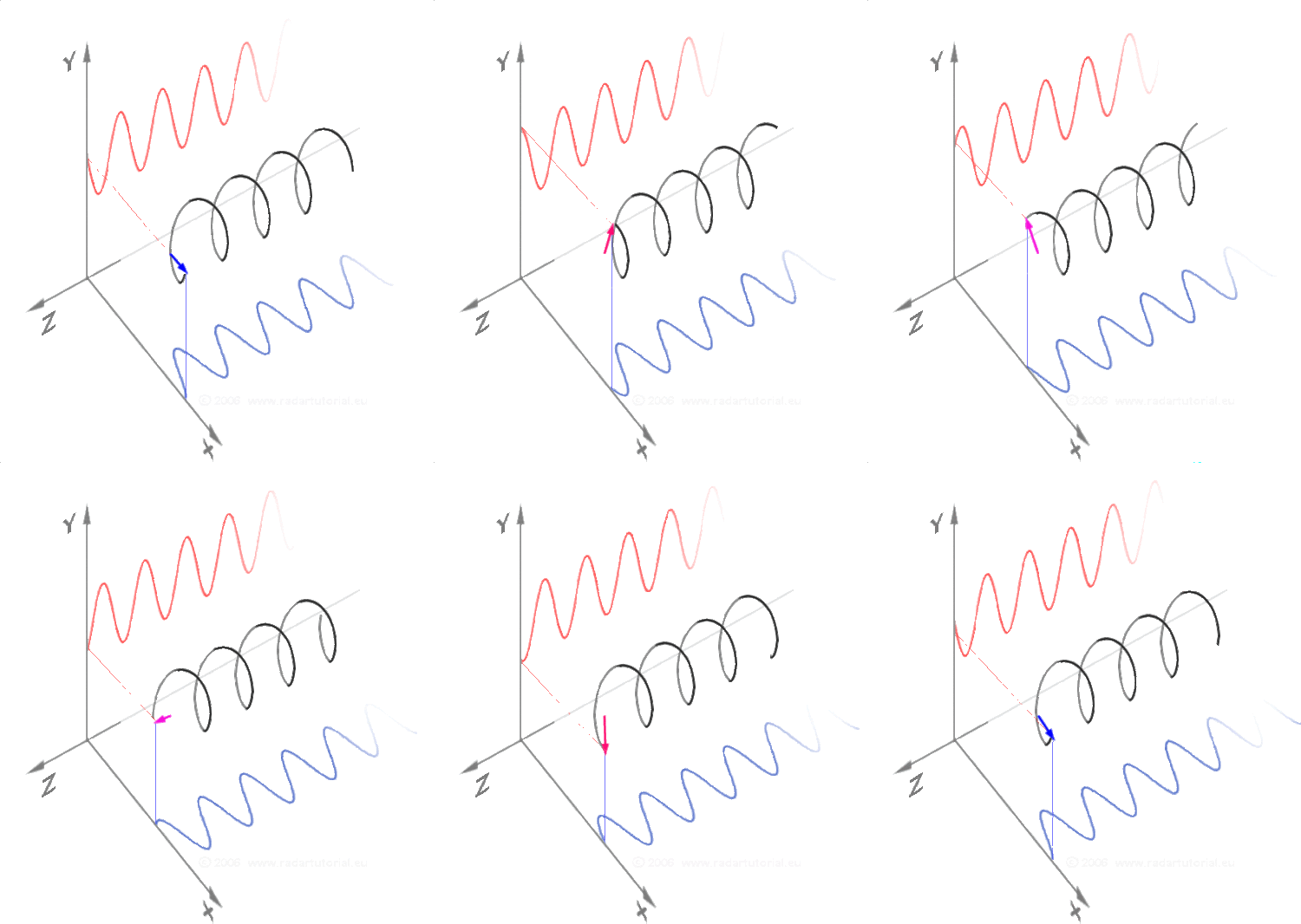
This awesome GIF is produced by RadarTutorial.eu, although I couldn't find it on their site. I originally found the image on this forum thread and the watermark bears RadarTutorial's site address (it's not too visible on the white background of this page).
Fourier
References
- An Interactive Guide To The Fourier Transform, BetterExplained.com
This is an awesome YouTube tutorial explaining how sine waves can be combined to produce any imaginable waveform:


